3.2. Quantum Amplitude Estimation of risk models#
For banks and insurances, modelling and assessing the business risk is an important task. A simple yet useful risk model was introduced and analyzed in the following article:
M. C. Braun, T. Decker, N. Hegemann, S. F. Kerstan, C. Schäfer: A Quantum Algorithm for the Sensitivity Analysis of Business Risks, arXiv:2103.05475.
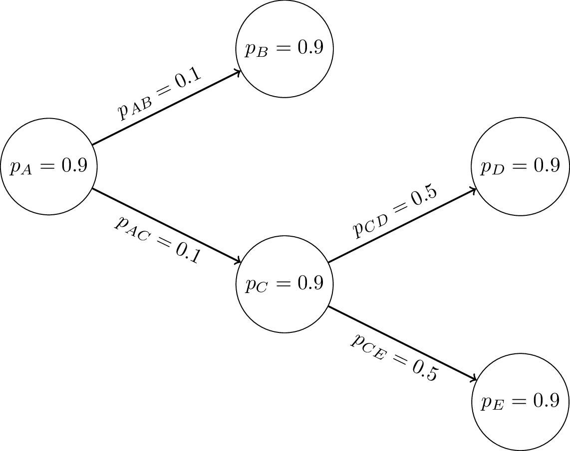
In this model, there are risk items like banks or companies with an associated probability of going bankrupt. These risk items are represented by nodes of a graph. The edges of the graph are the dependencies between the risk items: The bankruptcy of one risk item can lead to the bankruptcy of another risk item with a specified probability. In the following graph, a simple risk model with five risk items and several dependencies between them is shown:
 {width=350px}
In this diagram, the probability \(p_x\) is the probabilities that the corresponding node goes bankrupt and the probability \(p_{xy}\) is the probability that the bankruptcy of node \(x\) leads to the bankruptcy of node \(y\).
A risk model can be used to determine the probabilities of critical events like a loss, which goes beyond a pre-defined threshold. In many cases, risk models have a big number of risk items and many dependencies between them. This makes the analysis of some properties of such models a computationally hard task. To tackle such problems, a quantum version of such a risk model was developed and analyzed in the article cited above. To support and facilitate the development of quantum algorithms for evaluating such risk models, geqo is equipped with the RiskModel function to automatically convert a risk model to its quantum version.
The quantum version of a model is based on an efficient encoding, which uses one qubit per risk item. The probabilities and dependencies between the risk items are modelled by uncontrolled and controlled rotations, respectively. This efficient representation of risk models enables the evaluation of the risk model with the Grover algorithm and with Quantum Amplitude Estimation (QAE).
In the following, an example for a risk model is constructed with the geqo function RiskModel and the probability of an event is estimated with QAE.
3.2.1. Definition of the risk model#
As example, we consider the risk model from above with five risk items. In the dictionary probsNodes a probability is assigned to each nodes. This probability is the probability of a node to fail, e.g. the probability that a company goes bankrupt. The dictionary probsEdges contains edges with probability values. Each edge represents the probability that the failure of the first node in the edge causes the failure of the second node.
# defining the model
probsNodes = {
    "A": 0.9,
    "B": 0.9,
    "C": 0.9,
    "D": 0.9,
    "E": 0.9,
}  # intrinsic probabilities
probsEdges = {
    ("A", "B"): 0.1,
    ("A", "C"): 0.1,
    ("C", "D"): 0.5,
    ("C", "E"): 0.5,
}  # transition probabilities
With the geqo function RiskModel we can create a Sequence, which represents the quantum circuit corresponding to the risk model. This means that after running the circuit, the probability of measuring a configuration of failed or non-failed risk items corresponds exactly to the probability of this case. For instance, the probability for measuring the result 11111 is 0.6726 and this is the probability in the risk model that all risk items fail.
The function RiskModel returns a Sequence along with a dictionary of definitions of the BasicGates, which are used in the quantum circuit to set the values in the simulators.
from geqo.algorithms import RiskModel
from geqo.utils import embedSequences
from geqo.visualization import plot_mpl
from geqo.simulators import simulatorStatevectorNumpy

seq, cv = RiskModel(node_probs=probsNodes, edge_probs=probsEdges)
print("The Sequence corresponding to the risk model:")
print()
print(seq)
print()

sim = simulatorStatevectorNumpy(5, 5)
for c in cv:
    print("Definition of", c, ":")
    display(cv[c])
    sim.setValue(c, cv[c])

plot_mpl(embedSequences(seq), style="jos_dark", backend=sim)
The Sequence corresponding to the risk model:
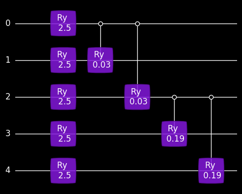
Sequence(['0', '1', '2', '3', '4'], [], [(Ry("Φ0"), ['0'], []), (Ry("Φ1"), ['1'], []), (QuantumControl([1], Ry("θ1")), ['0', '1'], []), (Ry("Φ2"), ['2'], []), (QuantumControl([1], Ry("θ2")), ['0', '2'], []), (Ry("Φ3"), ['3'], []), (QuantumControl([1], Ry("θ3")), ['2', '3'], []), (Ry("Φ4"), ['4'], []), (QuantumControl([1], Ry("θ4")), ['2', '4'], [])], "Risk")
Definition of Φ0 :
2.498091544796509
Definition of Φ1 :
2.498091544796509
Definition of θ1 :
0.034115800762489545
Definition of Φ2 :
2.498091544796509
Definition of θ2 :
0.034115800762489545
Definition of Φ3 :
2.498091544796509
Definition of θ3 :
0.19247429699702145
Definition of Φ4 :
2.498091544796509
Definition of θ4 :
0.19247429699702145
The model and the definition of the gates can be used to directly run the circuit on a simulator. In the following example, the SymPy based simulator is used to calculate the density matrix of the quantum system after applying the model. We display the entries on the diagonal of the density matrix, which are higher than 0.05; these entries correspond to the probability of measuring the corresponding result.
from geqo.operations import Measure

sim.apply(seq, [int(x) for x in seq.qubits])
sim.apply(Measure(5), [int(x) for x in seq.qubits], [int(x) for x in seq.qubits])
# sim.printQASM()

for r in sim.measurementResult:
    prob = sim.measurementResult[r]
    if prob > 0.05:
        print("-" * 20)
        print("r=", r, "has prob.", prob)
--------------------
r= (0, 1, 1, 1, 1) has prob. 0.07310249999999996
--------------------
r= (1, 0, 1, 1, 1) has prob. 0.0665232749999999
--------------------
r= (1, 1, 0, 1, 1) has prob. 0.05970509999999994
--------------------
r= (1, 1, 1, 1, 1) has prob. 0.6726242249999994
The last entry corresponds to the failure off all nodes and the corresponding probability of this event is \(0.6726\).
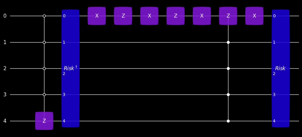
3.2.2. Construction of the Grover operator#
The Grover operator is composed as \(G=-R_Y(a) S_0 R_Y(-a) S_x\), where \(S_0\) and \(S_x\) are phase operations. More precisely, \(S_0\) multiplies the state \(|00000\rangle\) with the phase \(-1\) and all other states with the trivial phase \(1\). In a similar way, \(S_x\) marks the state \(|11111\rangle\) with \(-1\), for which we search the corresponding probability.
from geqo.operations import QuantumControl
from geqo.gates import PauliX, PauliZ
from geqo.core import Sequence

seqList = [
    (
        QuantumControl([1, 1, 1, 1], PauliZ()),
        ["0", "1", "2", "3", "4"],
        [],
    ),  # mark 11111 state
    (seq.getInverse(), ["0", "1", "2", "3", "4"], []),  # inverse operator
    (PauliX(), ["0"], []),  # the global -1
    (PauliZ(), ["0"], []),
    (PauliX(), ["0"], []),
    (PauliZ(), ["0"], []),
    (PauliX(), ["0"], []),  # Phase -1 on 0000 only, 1 else
    (QuantumControl([0, 0, 0, 0], PauliZ()), ["1", "2", "3", "4", "0"], []),
    (PauliX(), ["0"], []),
    (seq, ["0", "1", "2", "3", "4"], []),  # the operator
]

grov = Sequence(
    seq.qubits, seq.bits, seqList, "grov"
)  # Create the Grover operator as Sequence
plot_mpl(grov, style="jos_dark")
3.2.3. Construction of the QAE circuit#
For the QAE algorithm, we need the powers \(G, G^2, G^4, \ldots\) of the Grover operator. These powers are defined iteratively in the following.
grov = embedSequences(grov)
pow1 = Sequence(
    ["0", "1", "2", "3", "4"], [], [(grov, ["0", "1", "2", "3", "4"], [])], "G"
)
pow1 = embedSequences(pow1)
pow2 = Sequence(
    ["0", "1", "2", "3", "4"],
    [],
    [(pow1, ["0", "1", "2", "3", "4"], []), (pow1, ["0", "1", "2", "3", "4"], [])],
    "G2",
)
pow2 = embedSequences(pow2)
pow4 = Sequence(
    ["0", "1", "2", "3", "4"],
    [],
    [(pow2, ["0", "1", "2", "3", "4"], []), (pow2, ["0", "1", "2", "3", "4"], [])],
    "G4",
)
pow4 = embedSequences(pow4)
pow8 = Sequence(
    ["0", "1", "2", "3", "4"],
    [],
    [(pow4, ["0", "1", "2", "3", "4"], []), (pow4, ["0", "1", "2", "3", "4"], [])],
    "G8",
)
pow8 = embedSequences(pow8)
pow16 = Sequence(
    ["0", "1", "2", "3", "4"],
    [],
    [(pow8, ["0", "1", "2", "3", "4"], []), (pow8, ["0", "1", "2", "3", "4"], [])],
    "G16",
)
pow16 = embedSequences(pow16)
pow32 = Sequence(
    ["0", "1", "2", "3", "4"],
    [],
    [(pow16, ["0", "1", "2", "3", "4"], []), (pow16, ["0", "1", "2", "3", "4"], [])],
    "G32",
)
pow32 = embedSequences(pow32)
pow64 = Sequence(
    ["0", "1", "2", "3", "4"],
    [],
    [(pow32, ["0", "1", "2", "3", "4"], []), (pow32, ["0", "1", "2", "3", "4"], [])],
    "G64",
)
pow64 = embedSequences(pow64)
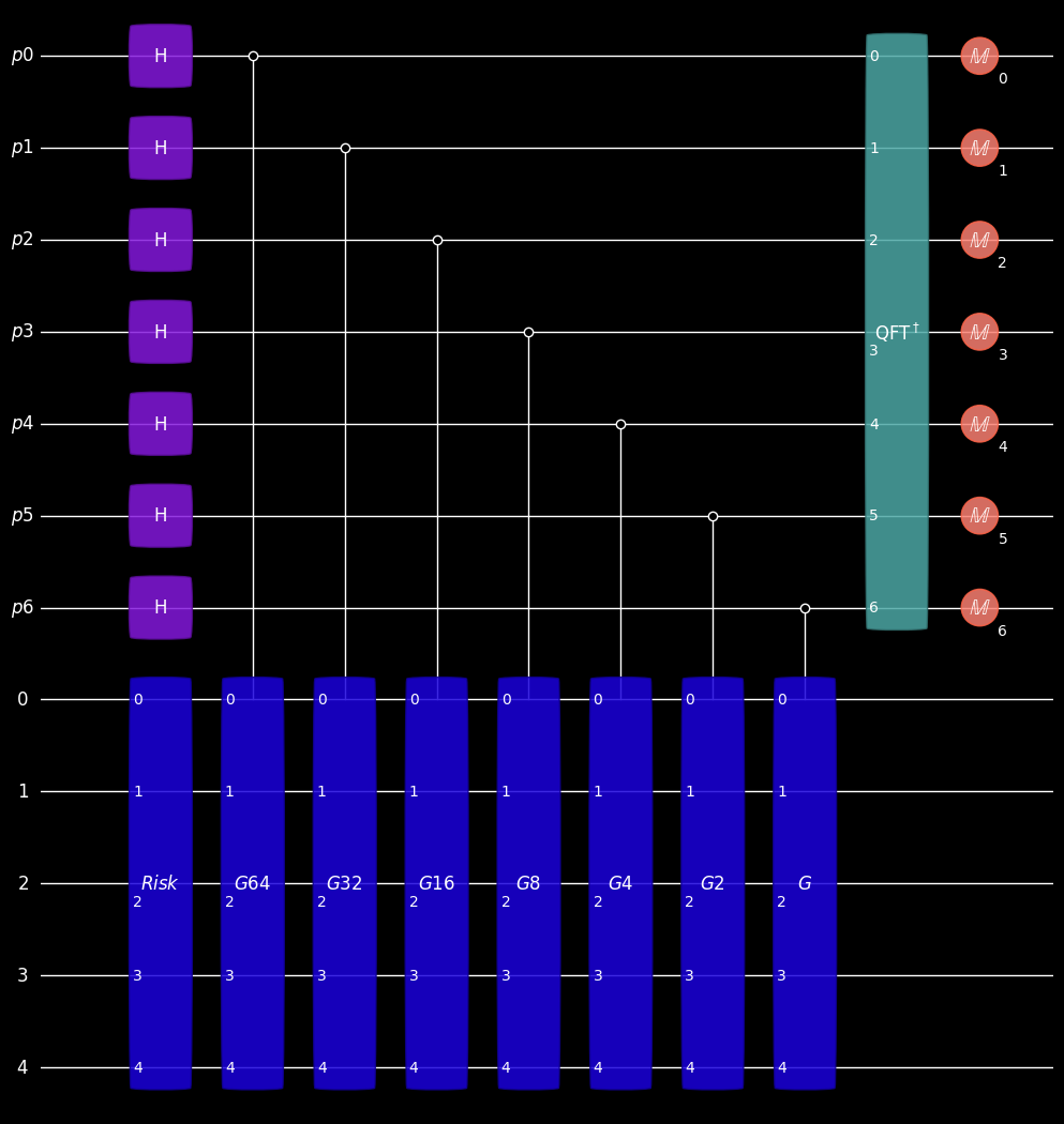
With the defined sequences, we can create the full circuit for the QAE. The qubits 0 to 4 are the working space for the risk model circuit and the Grover operators. The qubits p0 to p6 are initialized with a Hadamard transform and each is used for a phase kickback from a power of the Grover operator. At the end, an inverse QFT is applied to these qubits and they are measured in the standard basis. The result is a binary representation of the estimation of the probability, which corresponds to the event that all risk items have failed, i.e. the probability for measuring the state is \(|11111\rangle\).
from geqo.gates import Hadamard
from geqo.operations import QuantumControl
from geqo.algorithms import InverseQFT

qft = InverseQFT(7)
sim.prepareBackend([qft])

gatesAndTargets = []
for i in range(7):
    gatesAndTargets.append((Hadamard(), [f"p{i}"], []))

gatesAndTargets.append((seq, ["0", "1", "2", "3", "4"], []))

pows = [pow1, pow2, pow4, pow8, pow16, pow32, pow64]
for idx, p in enumerate(pows[::-1]):
    gatesAndTargets.append(
        (QuantumControl([1], p), [f"p{idx}", "0", "1", "2", "3", "4"], [])
    )

gatesAndTargets.append((qft, ["p0", "p1", "p2", "p3", "p4", "p5", "p6"], []))
gatesAndTargets.append((Measure(7), [f"p{i}" for i in range(7)], [*range(7)]))
qae = Sequence(
    ["p0", "p1", "p2", "p3", "p4", "p5", "p6", "0", "1", "2", "3", "4"],
    [*range(7)],
    gatesAndTargets,
)
plot_mpl(qae, style="jos_dark")
qae = embedSequences(qae)
# the QAE Sequence can be converted into qasm code
code = sim.sequence_to_qasm3(qae)
3.2.4. A function for evaluating the results of QAE#
The output of the QAE is an estimation of the probability in binary format. We define the function, which calculates the probability values corresponding to the binary outputs.
from geqo.utils import bin2num
import math


def bit2prob(bits):
    summe = bin2num(bits)
    res = summe / 2 ** (len(bits) - 1)
    theta_estim = math.pi * res / 2.0
    prob_estim = math.sin(theta_estim) * math.sin(theta_estim)
    return prob_estim
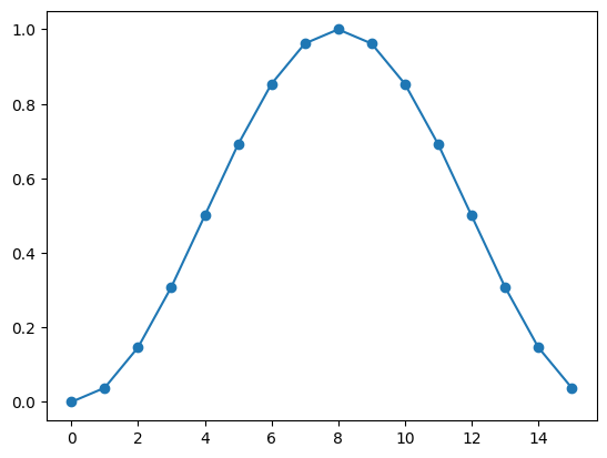
The probability values corresponding to the possible binary results are not evenly distributed in the intervall \([0,1]\). The following values and the plot shows that the values are denser around \(0\) and \(1\) in contrast to \(0.5\).
import itertools
import matplotlib.pyplot as plt

xe2 = []
ye2 = []
for i in itertools.product([0, 1], repeat=4):
    xe2.append(bin2num(i))
    ye2.append(bit2prob(i))
plt.scatter(xe2, ye2)
plt.plot(xe2, ye2)
[<matplotlib.lines.Line2D at 0x7f6199f50770>]
3.2.5. Running the QAE#
In the following, we use the NumPy based simulator simulatorStatevectorNumpy. Before we can run the QAE circuit and apply the measurements, the simulator has to be prepared with the methods setValue and prepareBackend. Since the RiskModel function returns matrix definitions in SymPy, we have to convert these matrices to NumPy with the function matrix2numpy.
from geqo.simulators.numpy import simulatorStatevectorNumpy

sim = simulatorStatevectorNumpy(12, 7)
for c in cv:
    print("setting c=", c)
    sim.setValue(c, cv[c])
sim.prepareBackend([qft])

sim.apply(qae, [*range(12)], [*range(7)])
setting c= Φ0
setting c= Φ1
setting c= θ1
setting c= Φ2
setting c= θ2
setting c= Φ3
setting c= θ3
setting c= Φ4
setting c= θ4
3.2.6. Results of the QAE#
The possible results of the measurement along with their corresponding probabilities are shown in the following. The results of the function bit2prob above shows that several binary results might correspond to the same probability estimation. Note that we only display results that have more than \(1\%\) probability.
te = {}
for ex in sim.measurementResult:
    e = [int(i) for i in list(ex)]
    estim = round(bit2prob(e), 5)
    prob = sim.measurementResult[ex]
    if prob > 0.01:
        print(
            "binary result: "
            + str(ex)
            + ", estimation: "
            + str(estim)
            + ", probability of this result: "
            + str(prob)
        )
    if estim in te:
        te[estim] += prob
    else:
        te[estim] = prob
binary result: (0, 1, 0, 0, 1, 1, 0), estimation: 0.64514, probability of this result: 0.010556852174544506
binary result: (0, 1, 0, 0, 1, 1, 1), estimation: 0.66844, probability of this result: 0.44831596084009684
binary result: (0, 1, 0, 1, 0, 0, 0), estimation: 0.69134, probability of this result: 0.02195105107156827
binary result: (1, 0, 1, 1, 0, 0, 0), estimation: 0.69134, probability of this result: 0.02195105107156827
binary result: (1, 0, 1, 1, 0, 0, 1), estimation: 0.66844, probability of this result: 0.44831596084009684
binary result: (1, 0, 1, 1, 0, 1, 0), estimation: 0.64514, probability of this result: 0.010556852174544508
The following plot shows the probability for each possible estimation of the probability of the event that all risk items have failed.
import matplotlib.pyplot as plt

xe = []
ye = []
maxIndex = 0
maxValue = 0
for t in te:
    xe.append(t)
    ye.append(te[t])
    if te[t] > maxValue:
        maxIndex = t
        maxValue = te[t]
# print(te)
print("result of QAE with highest probability:", maxIndex)
print("probability of this result:", maxValue)
plt.plot(xe, ye)
plt.scatter(xe, ye)
result of QAE with highest probability: 0.66844
probability of this result: 0.8966319216801937
<matplotlib.collections.PathCollection at 0x7f6199b11af0>
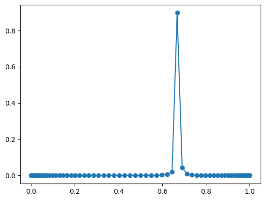
The result with the highest probability corresponds to the probability value \(0.66844\), which is the closest approximation to the probability \(0.6726\) for this level of precision. The probability of measuring this best approximation is over \(80\%\), i.e., the result can usually be found with two or three executions of the QAE circuit. The following diagram shows the concentration of the probability on the closest applroximation.